Fully-actuated vs Underactuated Systems
Many robots today move far too conservatively, and accomplish only a fraction of the tasks and achieve a fraction of the performance that they are mechanically capable of. In some cases, we are still fundamentally limited by control technology which matured on rigid robotic arms in structured factory environments, where large actuators could be used to "shape" the dynamics of the machine to achieve precision and repeatability. The study of underactuated robotics focuses on building control systems which instead exploit the natural dynamics of the machines in an attempt to achieve extraordinary performance in terms of speed, efficiency, or robustness.
In the last few years, controllers designed using machine learning have showcased the potential power of optimization-based control, but these methods do not yet enjoy the sample-efficiency nor algorithmic reliability that we've come to expect from more mature control technologies. The study of underactuated robotics asks us to look closely at the optimization landscapes that occur when we are optimizing mechanical systems, to understand and exploit that structure in our optimization and learning algorithms.
Motivation
Let's start with some examples, and some videos.
Honda's ASIMO vs. passive dynamic walkers
The world of robotics changed when, in late 1996, Honda Motor Co. announced that they had been working for nearly 15 years (behind closed doors) on walking robot technology. Their designs have continued to evolve, resulting in a humanoid robot they call ASIMO (Advanced Step in Innovative MObility). For nearly 20 years, Honda's robots were widely considered to represent the state of the art in walking robots, although there are now many robots with designs and performance very similar to ASIMO's. We will dedicate effort to understanding a few of the details of ASIMO when we discuss algorithms for walking... for now I just want you to become familiar with the look and feel of ASIMO's movements [watch the asimo video below now].
I hope that your first reaction is to be incredibly impressed with the
quality and versatility of ASIMO's movements. Now take a second look.
Although the motions are very smooth, there is something a little
unnatural about ASIMO's gait. It feels a little like an astronaut
encumbered by a heavy space suit. In fact this is a reasonable analogy...
ASIMO is walking a bit like somebody that is unfamiliar with his/her
dynamics. Its control system is using high-gain feedback, and therefore
considerable joint torque, to cancel out the natural dynamics of the
machine and strictly follow a desired trajectory. This control approach
comes with a stiff penalty. ASIMO uses roughly 20 times the energy
(scaled) that a human uses to walk on the flat (measured by cost of
transport)
For contrast, let's now consider a very different type of walking
robot, called a passive dynamic walker (PDW). This "robot" has no motors,
no controllers, no computer, but is still capable of walking stably down a
small ramp, powered only by gravity [watch videos above now]. Most people
will agree that the passive gait of this machine is more natural than
ASIMO's; it is certainly more efficient. Passive walking machines have a
long history - there are patents for passively walking toys dating back to
the mid 1800's. We will discuss, in detail, what people know about the
dynamics of these machines and what has been accomplished experimentally.
This most impressive passive dynamic walker to date was built by Steve
Collins in Andy Ruina's lab at Cornell
Passive walkers demonstrate that the high-gain, dynamics-cancelling feedback approach taken on ASIMO is not a necessary one. In fact, the dynamics of walking is beautiful, and should be exploited - not cancelled out.
The world is just starting to see what this vision could look like. This video from Boston Dynamics is one of my favorites of all time:
This result is a marvel of engineering (the mechanical design alone is amazing...). In this class, we'll teach you the computational tools required to make robots perform this way. We'll also try to reason about how robust these types of maneuvers are and can be. Don't worry: if you do not have a super lightweight, super capable, and super durable humanoid, then a simulation will be provided for you.
Birds vs. modern aircraft
The story is surprisingly similar in a very different type of machine. Modern airplanes are extremely effective for steady-level flight in still air. Propellers produce thrust very efficiently, and today's cambered airfoils are highly optimized for speed and/or efficiency. It would be easy to convince yourself that we have nothing left to learn from birds. But, like ASIMO, these machines are mostly confined to a very conservative, low angle-of-attack flight regime where the aerodynamics on the wing are well understood. Birds routinely execute maneuvers outside of this flight envelope (for instance, when they are landing on a perch), and are considerably more effective than our best aircraft at exploiting energy (eg, wind) in the air.
As a consequence, birds are extremely efficient flying machines; some
are capable of migrating thousands of kilometers with incredibly small
fuel supplies. The wandering albatross can fly for hours, or even days,
without flapping its wings - these birds exploit the shear layer formed by
the wind over the ocean surface in a technique called dynamic soaring.
Remarkably, the metabolic cost of flying for these birds is
indistinguishable from the baseline metabolic cost
Birds are also incredibly maneuverable. The roll rate of a highly
acrobatic aircraft (e.g, the A-4 Skyhawk) is approximately 720
deg/sec
Although many impressive statistics about avian flight have been
recorded, our understanding is partially limited by experimental
accessibility - it is quite difficult to carefully measure birds (and the
surrounding airflow) during their most impressive maneuvers without
disturbing them. The dynamics of a swimming fish are closely related, and
can be more convenient to study. Dolphins have been known to swim
gracefully through the waves alongside ships moving at 20
knots
Manipulation
Despite a long history of success in industrial applications, and the huge potential for consumer applications, we still don't have robot arms that can perform any meaningful tasks in the home. Admittedly, the perception problem (using sensors to detect/localize objects and understand the scene) for home robotics is incredibly difficult. But even if we were given a perfect perception system, our robots are still a long way from performing basic object manipulation tasks with the dexterity and versatility of a human.
Most robots that perform object manipulation today use a stereotypical pipeline. First, we enumerate a handful of contact locations on the hand (these points, and only these points, are allowed to contact the world). Then, given a localized object in the environment, we plan a collision-free trajectory for the arm that will move the hand into a "pre-grasp" location. At this point the robot closes it's eyes (figuratively) and closes the hand, hoping that the pre-grasp location was good enough that the object will be successfully grasped using e.g. only current feedback in the fingers to know when to stop closing. "Underactuated hands" make this approach more successful, but the entire approach really only works well for enveloping grasps.
The enveloping grasps approach may actually be sufficient for a number of simple pick-and-place tasks, but it is a very poor representation of how humans do manipulation. When humans manipulate objects, the contact interactions with the object and the world are very rich -- we often use pieces of the environment as fixtures to reduce uncertainty, we commonly exploit slipping behaviors (e.g. for picking things up, or reorienting it in the hand), and our brains don't throw NaNs if we use the entire surface of our arms to e.g. manipulate a large object.
In the last few years, the massive progress in computer vision has
completely opened up this space. I've began to focus my own research to
problems in the manipulation domain. In manipulation, the interaction
between dynamics and perception is incredibly rich. As a result, I've
started an entirely separate
set of notes (and a second course) on manipulation. That field, in
particular, feels like it is on the precipice: it seems clear that very
soon we will have some form of "foundation model"
By the way, in most cases, if the robots fail to make contact at the anticipated contact times/locations, bad things can happen. The results are hilarious and depressing at the same time. (Let's fix that!)
The common theme
Classical control techniques for robotics are based on the idea that feedback control can be used to override the dynamics of our machines. In contrast, the examples I've given above suggest that to achieve outstanding dynamic performance (efficiency, agility, and robustness) from our robots, we need to understand how to design control systems which take advantage of the dynamics, not cancel them out. That is the topic of this course.
Surprisingly, many formal control ideas that developed in robotics do not support the idea of "exploiting" the dynamics. Optimal control formulations (which we will study in depth) allow it in principle, but optimal control of nonlinear systems remains a challenging problem. Back when I started these notes, I used to joke that in order to convince a robotics control researcher to consider the dynamics, you have to do something drastic like taking away her control authority - remove a motor, or enforce a torque-limit. Systems that are interesting in this way are called the "underactuated" systems. It is in this field of "underactuated robotics" where research on the type of control I am advocating for began.
Definitions
According to Newton, the dynamics of mechanical systems are second order ($F = ma$). Their state is given by a vector of positions, $\bq$ (also known as the configuration vector), and a vector of velocities, $\dot{\bq}$, and (possibly) time. The general form for a second-order control dynamical system is: $$\ddot{\bq} = {\bf f}(\bq,\dot{\bq},\bu,t),$$ where $\bu$ is the control vector.
Underactuated Control Differential Equations
A second-order control differential equationAs we will see, the dynamics for many of the robots that we care about turn out to be affine in commanded torque (if $\bq$, $\dot{\bq}$, and $t$ are fixed, then the dynamics are a linear function of $\bu$ plus a constant), so let's consider a slightly constrained form: \begin{equation}\ddot{\bq} = {\bf f}_1(\bq,\dot{\bq},t) + {\bf f}_2(\bq,\dot{\bq},t)\bu \label{eq:f1_plus_f2}.\end{equation} For a control dynamical system described by equation \eqref{eq:f1_plus_f2}, if we have \begin{equation} \textrm{rank}\left[{\bf f}_2 (\bq,\dot{\bq},t)\right] < \dim\left[\bq\right],\label{eq:underactuated_low_rank}\end{equation} then the system is underactuated at $(\bq, \dot\bq, t)$. The implication is only in one direction, though -- sometimes we will write equations that look like \eqref{eq:f1_plus_f2} and have a full rank ${\bf f}_2$ but additional constraints like $|\bu|\le 1$ can also make a system underactuated.
Note also that we are using the word system here to describe the mathematical model (potentially of a physical robot). When we say that the system is underactuated, we are talking about the mathematical model. Imagine a two-link robot with two actuators, a typical model with rigid links could be fully actuated, but if we add extra degrees of freedom to model small amounts of flexibility in the links then that system model could be underactuated. These two models describe the same robot, but at different levels of fidelity. Two actuators might be enough to completely control the joint angles, but not the joint angles and the flexing modes of the link.
Notice that whether or not a control system is underactuated may depend on the state of the system or even on time, although for most systems (including all of the systems in this book) underactuation is a global property of the model. We will refer to a model as underactuated if it is underactuated in all states and times. In practice, we often refer informally to systems as fully actuated as long as they are fully actuated in most states (e.g., a "fully-actuated" system might still have joint limits or lose rank at a kinematic singularity). Admittedly, this permits the existence of a gray area, where it might feel awkward to describe the model as either fully- or underactuated (we should instead only describe its states); even powerful robot arms on factory floors do have actuator limits, but we can typically design controllers for them as though they were fully actuated. The primary interest of this text is in models for which the underactuation is useful/necessary for developing a control strategy.
Robot Manipulators

Consider the simple robot manipulator illustrated above. As described in the Appendix, the equations of motion for this system are quite simple to derive, and take the form of the standard "manipulator equations": $${\bf M}(\bq)\ddot\bq + \bC(\bq,\dot\bq)\dot\bq = \btau_g(\bq) + {\bf B}\bu.$$ It is well known that the inertia matrix, ${\bf M}(\bq)$ is (always) uniformly symmetric and positive definite, and is therefore invertible. Putting the system into the form of equation \ref{eq:f1_plus_f2} yields: \begin{align*}\ddot{\bq} =& {\bf M}^{-1}(\bq)\left[ \btau_g(\bq) + \bB\bu - \bC(\bq,\dot\bq)\dot\bq \right].\end{align*} Because ${\bf M}^{-1}(\bq)$ is always full rank, we find that a system described by the manipulator equations is fully actuated if and only if $\bB$ is full row rank. For this particular example, $\bq = [\theta_1,\theta_2]^T$ and $\bu = [\tau_1,\tau_2]^T$ (motor torques at the joints), and ${\bf B} = {\bf I}_{2 \times 2}$. The system is fully actuated.
I personally learn best when I can experiment and get some physical intuition. Most chapters in these notes have an associated Jupyter notebook that can run on Deepnote; this chapter's notebook makes it easy for you to see this system in action.
Try it out! You'll see how to simulate the double pendulum, and even how to inspect the dynamics symbolically.
Note: You can also run the code on your own machines (see the Appendix for details).
While the basic double pendulum is fully actuated, imagine the somewhat bizarre case that we have a motor to provide torque at the elbow, but no motor at the shoulder. In this case, we have $\bu = \tau_2$, and $\bB(\bq) = [0,1]^T$. This system is clearly underactuated. While it may sound like a contrived example, it turns out that it is almost exactly the dynamics we will use to study as our simplest model of walking later in the class.
The matrix ${\bf f}_2$ in equation \ref{eq:f1_plus_f2} always has dim$[\bq]$ rows, and dim$[\bu]$ columns. Therefore, as in the example, one of the most common cases for underactuation, which trivially implies that ${\bf f}_2$ is not full row rank, is dim$[\bu] < $ dim$[\bq]$. This is the case when a robot has joints with no motors. But this is not the only case. The human body, for instance, has an incredible number of actuators (muscles), and in many cases has multiple muscles per joint; despite having more actuators than position variables, when I jump through the air, there is no combination of muscle inputs that can change the ballistic trajectory of my center of mass (barring aerodynamic effects). My control system is underactuated.
A quick note about notation. When describing the dynamics of rigid-body systems in this class, I will use $\bq$ for configurations (positions), $\dot{\bq}$ for velocities, and use $\bx$ for the full state ($\bx = [\bq^T,\dot{\bq}^T]^T$). There is an important limitation to this convention (3D angular velocity should not be represented as the derivative of 3D pose) described in the Appendix, but it will keep the notes cleaner. Unless otherwise noted, vectors are always treated as column vectors. Vectors and matrices are bold (scalars are not).
Feedback Equivalence
Fully-actuated systems are dramatically easier to control than underactuated systems. The key observation is that, for fully-actuated systems with known dynamics (e.g., ${\bf f}_1$ and ${\bf f}_2$ are known for a second-order control-affine system), it is possible to use feedback to effectively change an arbitrary control problem into the problem of controlling a trivial linear system.
When ${\bf f}_2$ is full row rank, it has a right inverse
Feedback Cancellation on the Double Pendulum
Let's say that we would like our simple double pendulum to act like a
simple single pendulum (with damping), whose dynamics are given by:
\begin{align*} \ddot \theta_1 &= -\frac{g}{l}\sin\theta_1 -b\dot\theta_1 \\
\ddot\theta_2 &= 0. \end{align*} This is easily achieved using
Since we are embedding a nonlinear dynamics (not a linear one), we refer to this as "feedback cancellation", or "dynamic inversion". This idea reveals why I say control is easy -- for the special case of a fully-actuated deterministic system with known dynamics. For example, it would have been just as easy for me to invert gravity. Observe that the control derivations here would not have been any more difficult if the robot had 100 joints.
You can run these examples in the notebook:
As always, I highly recommend that you take a few minutes to read through the source code.
Fully-actuated systems are feedback equivalent to $\ddot\bq = \bu$, whereas underactuated systems are not feedback equivalent to $\ddot\bq = \bu$. Therefore, unlike fully-actuated systems, the control designer has no choice but to reason about the more complex dynamics of the plant in the control design. When these dynamics are nonlinear, this can dramatically complicate feedback controller design.
A related concept is feedback linearization. The feedback-cancellation controller in the example above is an example of feedback linearization -- using feedback to convert a nonlinear system into a controllable linear system. Asking whether or not a system is "feedback linearizable" is not the same as asking whether it is underactuated; even a controllable linear system can be underactuated, as we will discuss soon.
Perhaps you are coming with a background in optimization or machine learning, rather than linear controls? To you, I could say that for fully-actuated systems, there is a straight-forward change of variables that can make the optimization landscape (for many control performance objectives) convex. Optimization/learning for these systems is relatively easy. For underactuated systems, we can still aim to leverage the mechanics to improve the optimization landscape but it requires more insights. Developing those insights is one of the themes in these notes, and continues to be an active area of research.
Input and State Constraints
Although the dynamic constraints due to missing actuators certainly embody the spirit of this course, many of the systems we care about could be subject to other dynamic constraints as well. For example, the actuators on our machines may only be mechanically capable of producing some limited amount of torque, or there may be a physical obstacle in the free space with which we cannot permit our robot to come into contact with.
Input and State Constraints
A dynamical system described by $\dot{\bx} = {\bf f}(\bx,\bu,t)$ may be subject to one or more constraints described by $\bphi(\bx,\bu,t)\ge0$.In practice it can be useful to separate out constraints which depend only on the input, e.g. $\phi(\bu)\ge0$, such as actuator limits, as they can often be easier to handle than state constraints. An obstacle in the environment might manifest itself as one or more constraints that depend only on position, e.g. $\phi(\bq)\ge0$.
By our generalized definition of underactuation, we can see that input constraints can certainly cause a system to be underactuated. Position equality constraints are more subtle -- in general these actually reduce the dimensionality of the state space, therefore requiring less dimensions of actuation to achieve "full" control, but we only reap the benefits if we are able to perform the control design in the "minimal coordinates" (which is often difficult).
Input limits
Consider the constrained second-order linear system \[ \ddot{x} = u, \quad |u| \le 1. \] By our definition, this system is underactuated. For example, there is no $u$ which can produce the acceleration $\ddot{x} = 2$.Input and state constraints can complicate control design in similar ways to having an insufficient number of actuators, (i.e., further limiting the set of the feasible trajectories), and often require similar tools to find a control solution.
Nonholonomic constraints
You might have heard of the term "nonholonomic system" (see e.g.
Wheeled robot
Consider a simple model of a wheeled robot whose configuration is described by its Cartesian position $x,y$ and its orientation, $\theta$, so $\bq = \begin{bmatrix} x, y, \theta \end{bmatrix}^T$. The system is subject to a differential constraint that prevents side-slip, \begin{gather*} \dot{x} = v \cos\theta \\ \dot{y} = v \sin\theta \\ v = \sqrt{\dot{x}^2 + \dot{y}^2} \end{gather*} or equivalently, \[\dot{y} \cos \theta - \dot x \sin \theta = 0.\] This constraint cannot be integrated into a constraint on configuration—the car can get to any configuration $(x,y,\theta)$, it just can't move directly sideways—so this is a nonholonomic constraint.Contrast the wheeled robot example with a robot on train tracks. The train tracks correspond to a holonomic constraint: the track constraint can be written directly in terms of the configuration $\bq$ of the system, without using the velocity ${\bf \dot{q}}$. Even though the track constraint could also be written as a differential constraint on the velocity, it would be possible to integrate this constraint to obtain a constraint on configuration. The track restrains the possible configurations of the system.
A nonholonomic constraint like the no-side-slip constraint on the wheeled vehicle certainly results in an underactuated system. The converse is not necessarily true—the double pendulum system which is missing an actuator is underactuated but would not typically be called a nonholonomic system. Note that the Lagrangian equations of motion are a constraint of the form \[\bphi(\bq,\dot\bq, \ddot\bq, \bu, t) = 0,\] so do fit our simple form for a first-order nonholonomic constraint.
Underactuated robotics
Today, control design for underactuated systems relies heavily on optimization and optimal control, with fast progress but still many open questions in both model-based optimization and machine learning for control. It's a great time to be studying this material! Now that computer vision has started to work, and we can ask large language models for high-level instructions what our robot should be doing (e.g. "chat GPT, give me detailed instructions on how to make a pizza"), we still have many interesting problems in robotics that are still hard because they are underactuated:
- Legged robots are underactuated. Consider a legged machine with $N$ internal joints and $N$ actuators. If the robot is not bolted to the ground, then the degrees of freedom of the system include both the internal joints and the six degrees of freedom which define the position and orientation of the robot in space. Since $\bu \in \Re^N$ and $\bq \in \Re^{N+6}$, equation \eqref{eq:underactuated_low_rank} is satisfied.
- (Most) Swimming and flying robots are underactuated. The story is the same here as for legged machines. Each control surface adds one actuator and one DOF. And this is already a simplification, as the true state of the system should really include the (infinite-dimensional) state of the flow.
- Robot manipulation is (often) underactuated. Consider a fully-actuated robotic arm. When this arm is manipulating an object with degrees of freedom (even a brick has six), it can become underactuated. If force closure is achieved, and maintained, then we can think of the system as fully-actuated, because the degrees of freedom of the object are constrained to match the degrees of freedom of the hand. That is, of course, unless the manipulated object has extra DOFs (for example, any object that is deformable).
Being underactuated changes the approach we take for planning and control. For instance, if you look at the chapter on trajectory optimization in these notes, and compare them to the chapter on trajectory optimization in my manipulation notes, you will see that they formulate the problem quite differently. For a fully-actuated robot arm, we can focus on planning kinematic trajectories without immediately worrying about the dynamics. For underactuated systems, one must worry about the dynamics.
Even control systems for fully-actuated and otherwise unconstrained systems can be improved using the lessons from underactuated systems, particularly if there is a need to increase the efficiency of their motions or reduce the complexity of their designs.
Goals for the course
This course studies the rapidly advancing computational tools from optimization theory, control theory, motion planning, and machine learning which can be used to design feedback control for underactuated systems. The goal of this class is to develop these tools in order to design robots that are more dynamic and more agile than the current state-of-the-art.
The target audience for the class includes both computer science and mechanical/aero students pursuing research in robotics. Although I assume a comfort with linear algebra, ODEs, and Python, the course notes aim to provide most of the material and references required for the course.
I have a confession: I actually think that the material we'll cover in these notes is valuable far beyond robotics. I think that systems theory provides a powerful language for organizing computation in exceedingly complex systems -- especially when one is trying to program and/or analyze systems with continuous variables in a feedback loop (which happens throughout computer science and engineering, by the way). I hope you find these tools to be broadly useful, even if you don't have a humanoid robot capable of performing a backflip at your immediate disposal.
Exercises
Atlas Backflip
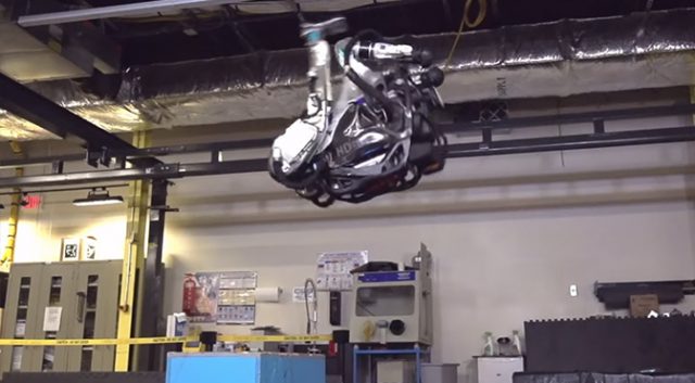
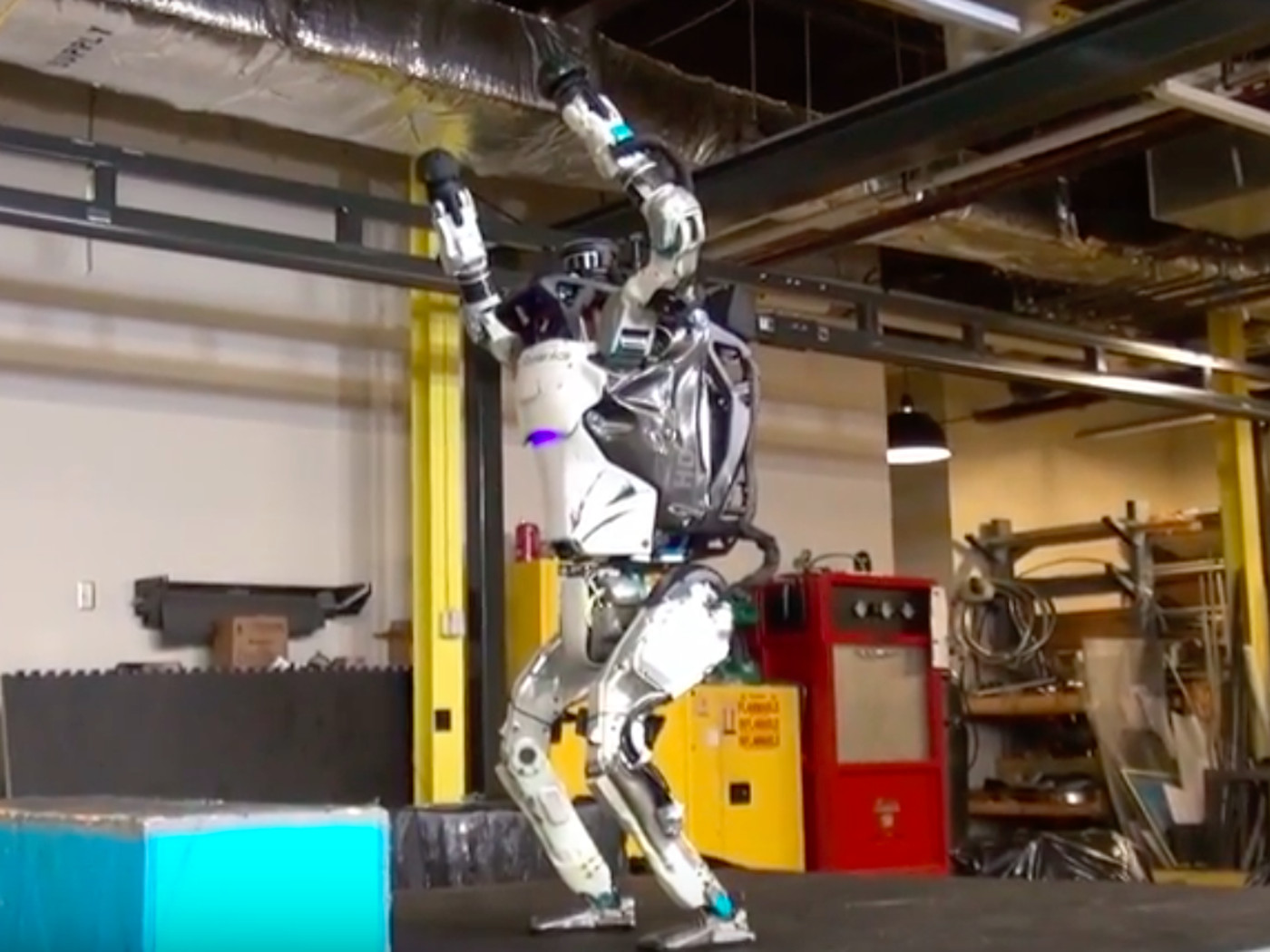
- The state of the humanoid can be represented by the angles and the angular velocities of all its joints.
- While doing the backflip (state in the left figure), the humanoid is fully actuated.
- While standing (state in the right figure), the humanoid is fully actuated.
Trajectory Tracking in State Space
Take a robot whose dynamics is governed by equation \ref{eq:f1_plus_f2}, and assume it to be fully actuated in all states $\bx = [\bq^T, \dot\bq^T]^T$ at all times $t$.- For any twice-differentiable desired trajectory $\bq_{\text{des}}(t)$, is it always possible to find a control signal $\bu(t)$ such that $\bq(t) = \bq_{\text{des}}(t)$ for all $t \geq 0$, provided that $\bq(0) = \bq_{\text{des}}(0)$ and $\dot \bq(0) = \dot \bq_{\text{des}}(0)$?
- Now consider the simplest fully-actuated robot: the double integrator. The dynamics of this system reads $m \ddot q = u$, and you can think of it as a cart of mass $m$ moving on a straight rail, controlled by a force $u$. The figure below depicts its phase portrait when $u=0$. Is it possible to find a control signal $u(t)$ that drives the double integrator from the initial state $\bx(0) = [2, 0.5]^T$ to the origin along a straight line (blue trajectory)? Does the answer change if we set $\bx(0)$ to be $[2, -0.5]^T$ (red trajectory)?

Phase portrait of the double integrator. - The dynamics \ref{eq:f1_plus_f2} are $n=\dim[\bq]$ second-order differential equations. However, it is always possible (and we'll frequently do it) to describe these equations in terms of $2n$ first-order differential equations $\dot \bx = f(\bx,t)$. To this end, we simply define $$f(\bx,t) = \begin{bmatrix} \dot\bq \\ {\bf f}_1(\bq,\dot\bq,t) + {\bf f}_2(\bq,\dot\bq,t)\bu \end{bmatrix}.$$ For any twice-differentiable trajectory $\bx_{\text{des}}(t)$, is it always possible to find a control $\bu(t)$ such that $\bx(t) = \bx_{\text{des}}(t)$ for all $t \geq 0$, provided that $\bx(0) = \bx_{\text{des}}(0)$?
Task-Space Control of the Double Pendulum
In the example above, we have seen that the double pendulum with one motor per joint is a fully-actuated system. Here we consider a variation of it: instead of controlling the robot with the actuators at the shoulder and the elbow, we directly apply a force on the mass $m_2$ (tip of the second link). Let $\bu = [u_1, u_2]^T$ be this force, with $u_1$ horizontal component (positive to the right) and $u_2$ vertical component (positive upwards). This modification leaves the equations of motion derived in the appendix example almost unchanged; the only difference is that the matrix $\bB$ is now a function of $\bq$. Namely, using the notation from the appendix, $$\bB (\bq) = \begin{bmatrix} l_1 c_1 + l_2 c_{1+2} & l_1 s_1 + l_2 s_{1+2} \\ l_2 c_{1+2} & l_2 s_{1+2} \end{bmatrix}.$$ Is the double pendulum with the new control input still fully-actuated in all states? If not, identify the states in which it is underactuated.Underactuation of the Planar Quadrotor
Later in the course we will study the dynamics of a quadrotor quite in depth, for the moment just look at the structure of the resulting equations of motion from the planar quadrotor section. The quadrotor is constrained to move in the vertical plane, with the gravity pointing downwards. The configuration vector $\bq = [x, y, \theta]^T$ collects the position of the center of mass and the pitch angle. The control input is the thrust $\bu = [u_1, u_2]^T$ produced by the two rotors. The input $\bu$ can assume both signs and has no bounds.- Identify the set of states $\bx = [\bq^T, \dot \bq^T]^T$ in which the system is underactuated.
- For all the states in which the system is underactuated, identify an acceleration $\ddot \bq (\bq, \dot \bq)$ that cannot be instantaneously achieved. Provide a rigorous proof of your claim by using the equations of motion: plug the candidate accelerations in the dynamics, and try to come up with contradictions such as $mg=0$.
Drake Systems
The course software, Drake, provides a powerful modeling language for dynamical systems. The exercise in will help you write your first Drake System.