System Identification
My primary focus in these notes has been to build algorithms that design of analyze a control system given a model of the plant. In fact, we have in some places gone to great lengths to understand the structure in our models (the structure of the manipulator equations in particular) and tried to write algorithms which exploit that structure.
Our ambitions for our robots have grown over recent years to where it makes sense to question this assumption. If we want to program a robot to fold laundry, spread peanut butter on toast, or make a salad, then we should absolutely not assume that we are simply given a model (and the ability to estimate the state of that model). This has led many researchers to focus on the "model-free" approaches to optimal control that are popular in reinforcement learning. But I worry that the purely model-free approach is "throwing the baby out with the bathwater". We have fantastic tools for making long-term decisions given a model; the model-free approaches are correspondingly much much weaker.
So in this chapter I would like to cover the problem of learning a model. This is far from a new problem. The field of "system identification" is as old as controls itself, but new results from machine learning have added significantly to our algorithms and our analyses, especially in the high-dimensional and finite-sample regimes. But well before the recent machine learning boom, system identification as a field had a very strong foundation with thorough statistical understanding of the basic algorithms, at least in the asymptotic regime (the limit where the amount of data goes to infinity). Machine learning theory has brought a wealth of new results in the online optimization and finite-sample regimes. My goal for this chapter is to establish these foundations, and to provide some pointers so that you can learn more about this rich topic.
Problem formulation
Equation error vs simulation error

Our problem formulation inevitably begins with the data. In practice, if we have access to a physical system, instrumented using digital electronics, then we have a system in which we can apply input commands, $\bu_n$, at some discrete rate, and measure the outputs, $\by_n$ of the system at some discrete rate. We normally assume these rates our fixed, and often attempt to fit a state-space model of the form \begin{equation} \bx[n+1] = f_\balpha(\bx[n], \bu[n]), \qquad \by[n] = g_\balpha(\bx[n],\bu[n]), \label{eq:ss_model}\end{equation} where I have used $\balpha$ again here to indicate a vector of parameters. In this setting, a natural formulation is to minimize a least-squares estimation objective: $$\min_{\alpha,\bx[0]} \sum_{n=0}^{N-1} \| \by[n] - \by_n \|^2_2, \qquad \subjto \, (\ref{eq:ss_model}).$$ I have written purely deterministic models to start, but in general we expect both the state evolution and the measurements to have randomness. Sometimes, as I have written, we fit a deterministic model to the data and rely on our least-squares objective to capture the errors; more generally we will look at fitting stochastic models to the data.
We often separate the identification procedure into two parts, in which we first estimate the state $\hat{\bx}_n$ given the input-output data $\bu_n, \by_n$, and then focus on estimating the state-evolution dynamics in a second step. The dynamics estimation algorithms fall into two main categories:
- Equation error minimizes only the one-step prediction error: $$\min_{\alpha} \sum_{n=0}^{N-2} \| f_\balpha(\hat\bx_n, \bu_n) - \hat{\bx}_{n+1} \|^2_2.$$
- Simulation error captures the long-term prediction error: $$\min_{\alpha} \sum_{n=1}^{N-1} \| \bx[n] - \hat{\bx}_n \|^2_2, \qquad \subjto \quad \bx[n+1] = f_\balpha(\bx[n], \bu_n),\, \bx[0] = \hat\bx_0,$$
Within this framework of model learning, we will face all of the standard questions from supervised learning about sample efficiency and generalization.
Online optimization
Theoretical machine learning has brought a number of fresh
perspectives to this old problem of system identification. Perhaps most
relevant is the perspective of online optimization
In the regret formulation, we acknowledge that the class of parameterized models that we are searching over can likely not perfectly represent the input-output data. Rather than score ourselves directly on the prediction error, we can score ourselves relative to the predictions that would be made by best parameters in our model class. For equation-error formulations, the regret $R$ at step $N$ would take the form $$R[N] = \sum_{n=0}^{N-2} \| f_\balpha(\hat\bx_n, \bu_n) - \hat{\bx}_{n+1} \|^2_2 - \min_{\alpha^*} \sum_{n=0}^{N-2} \| f_{\alpha^*}(\hat\bx_n, \bu_n) - \hat{\bx}_{n+1} \|^2_2.$$ The goal is to produce an online learning algorithm to select $\alpha$ at each step in order to drive the regret to zero. This turns out to be an important distinction, as we will see below.
Learning models for control
So far we've described the problem purely as capturing the input-output behavior of the system. If our goal is to use this model for control, then that might not be quite the right objective for a number of reasons.
First of, predicting the observations might be more than we
need for making optimal decisions;
There are other considerations, as well. To be useful for control,
we'll need the state of our model to be observable (from online
observations) and controllable. There may also be trade-offs in model
complexity. If we learn a just linear model of the dynamics then we have
very powerful control design tools available, but we might not capture
the rich dynamics of the world. If we learn too complex of a model, then
our online planning and control techniques might become a bottleneck.
Parameter Identification for Mechanical Systems
My primary focus throughout these notes is on (underactuated) mechanical systems, but when it comes to identification there is an important distinction to make. For some mechanical systems we know the structure of the model, including number of state variables and the topology of the kinematic tree. Legged robots like Spot or Atlas are good examples here -- the dynamics are certainly nontrivial, but the general form of the equations are known. In this case, the task of identification is really the task of estimating the parameters in a structured model. That is the subject of this section.
The examples of folding laundry or making a salad fall into a different category. In those examples, I might not even know a priori the number of state variables needed to provide a reasonable description of the behavior. That will force a more general examination of the the identification problem, which we will explore in the remaining sections.
Let's start with the problem of identifying a canonical underactuated mechanical system, like an Acrobot, Cart-Pole or Quadrotor, where we know the structure of the equations, but just need to fit the parameters. We will further assume that we have the ability to directly observe all of the state variables, albeit with noisy measurements (e.g. from joint sensors and/or inertial measurement units). The stronger state estimation algorithms that we will discuss soon assume a model, so we typically do not use them directly here.
Consider taking a minute to review the example of deriving the manipulator equations for the double pendulum before we continue.
Kinematic parameters and calibration
We can separate the parameters in the multibody equations again into
kinematic parameters and dynamic parameters. The kinematic parameters,
like link lengths, describe the coordinate transformation from one joint
to another joint in the kinematic tree. It is certainly possible to
write an optimization procedure to calibrate these parameters; you can
find a fairly thorough discussion in e.g. Chapter 11 of
One notable exception to this is calibration with respect to joint offsets. This one can be a real nuisance in practice. Joint sensors can slip, and some robots even use relative rotary encoders, and rely on driving the joint to some known hard joint limit each time the robot is powered on in order to obtain the offset. I've worked on one advanced robot that had a quite elaborate and painful kinematic calibration procedure which involve fitting additional hardware over the joints to ensure they were in a known location and then running a script. Having an expensive and/or unreliable calibration procedure can put a damper on any robotics project.
Acrobot balancing with calibration error
Small kinematic calibration errors can lead to large steady-state errors when attempting to stabilize a system like the Acrobot. I've put together a simple notebook to show the effect here:
Our tools from robust / stochastic control are well-suited to identifying (and bounding / minimizing) these sensitivities, at least for the linearized model we use in LQR.
The general approach to estimating joint offsets from data is to write the equations with the joint offset as a parameter, e.g. for the double pendulum we would write the forward kinematics as: $${\bf p}_1 =l_1\begin{bmatrix} \sin(\theta_1 + \bar\theta_1) \\ - \cos(\theta_1 + \bar\theta_1) \end{bmatrix},\quad {\bf p}_2 = {\bf p}_1 + l_2\begin{bmatrix} \sin(\theta_1 + \bar\theta_1 + \theta_2 + \bar\theta_2) \\ - \cos(\theta_1 + \bar\theta_1 + \theta_2 + \bar\theta_2) \end{bmatrix}.$$ We try to obtain independent measurements of the end-effector position (e.g. from motion capture, from perhaps some robot-mounted cameras, or from some mechanical calibration rig) with their corresponding joint measurements, to obtain data points of the form $ \langle {\bf p}_2, \theta_1, \theta_2 \rangle$. Then we can solve a small nonlinear optimization problem to estimate the joint offsets to minimize a least-squares residual.
If independent measurements of the kinematics are not available, it it possible to estimate the offsets along with the dynamic parameters, using the trigonometric identities, e.g. $s_{\theta + \bar\theta} = s_\theta c_\bar\theta + c_\theta s_\bar\theta,$ and then including the $s_\bar\theta, c_\bar\theta$ terms (separately) in the "lumped parameters" we discuss below.
Estimating inertial parameters (and friction)
Now let's think about estimating the inertial parameters of
multibody system. We've been writing the manipulation equations in the
form: \begin{equation}\bM({\bq})\ddot{\bq} + \bC(\bq,\dot{\bq})\dot\bq =
\btau_g(\bq) + \bB\bu + \text{friction, etc.}\end{equation} Each of the
terms in this equation can depend on the parameters $\balpha$ that we're
trying to estimate. But the parameters enter the multibody equations in
a particular structured way: the inverse dynamics equations are
affine in the inertial parameters
To proceed with the inverse dynamics formulation, let us first choose
a parameterization for the inertias.
Remarkably, the inverse dynamics are affine in these parameters. This
means that the manipulator equations above can be refactored into the
form \begin{equation}{\bf W}(\bq_n,\dot{\bq}_n, \ddot{\bq}_n, \bu_n)
\balpha_B + \bw_0(\bq_n,\dot{\bq}_n, \ddot{\bq}_n, \bu_n) = 0.
\label{eq:least_squares}\end{equation} We sometimes refer to the ${\bf
W}$ which is assembled by vertically stacking these equations evaluated
at all time samples, $n$, as the "data matrix". Given data trajectories
of positions, $\bq_n,$ and torque measurements, $\bu_n,$ we can estimate
$\dot{\bq}_n$ and $\ddot{\bq}_n$ with (acausal) filtering. Then we can
estimate the parameters using least-squares estimation. As such, we can
leverage all of the strong results and variants from linear estimation.
For instance, we can add terms to regularize the estimate (e.g. to stay
close to an initial guess), and we can write efficient recursive
estimators for optimal online estimation of the parameters using
recursive least-squares. My favorite recursive least-squares algorithm
uses incremental QR factorization
Not all values of $\alpha_B$ describe physically-valid inertias. For
instance, we know that $m_B$ has to be positive. There are constraints on
the inertia matrix itself.
Do these additional constraints matter? In the limit of infinite data, then one might hope that the least-squares estimator would obtain the correct values without the constraints. But their are two foils to this ideal. First, we often wish to operate in a relatively low-data regime. Second, it is important to understand that not all of the inertial parameters will be identifiable. For instance, if you imagine a robotic arm bolted to a table where the first link is a rotation about the $z$ axis. Then no amount of data obtained from this robot will given any information about the moments of inertia of the first link about the $x$ and $y$ axes. Naively including these parameters in the estimation problem could not only lead to poor estimates of the unidentifiable parameters, but can even render the physical-validity constraints on the inertial parameters vacuous.
There are two general approaches to dealing with the unidentifiable
parameters. First, we can exclude them from the optimization. There are a
number of algorithms for symbolically extracting the identifiable
parameters, but it is more common (and likely just as effective) to
simply evaluate the null-space of a sufficiently rich data matrix, $W$,
to find the unidentifiable parameters by using, e.g., $\bR_1\alpha_l$
from the QR factorization: $${\bf W} = \begin{bmatrix} \bQ_1 & \bQ_2
\end{bmatrix} \begin{bmatrix} \bR_1 \\ 0 \end{bmatrix}, \quad \Rightarrow
\quad {\bf W}\balpha_B = \bQ_1 (\bR_1 \balpha_B) = \bQ_1
\bar{\balpha}_{B},$$ where $\bar{\balpha}_B$ are the identifiable
parameters. To implement the physical-validity constraints, we would need
to use estimates of the unidentifiable parameters. Alternatively, one
can formulate the optimization directly on the full parameters and add a
regularization term which (ideally) operates in the nullspace of the
primary objective to drive the unidentifiable parameters towards a prior
estimate.
The least-squares inverse-dynamics formulation also allows one to simultaneously fit a number of other relevant dynamic parameters which enter linearly into the equations. These include reflected inertial (as a diagonal matrix times $\ddot{\bq}$), joint friction (as a constant torque multiplied by the sign of $\dot{\bq}$), and damping (as a linear multiple of $\dot{\bq}$).
Allow me to mention one subtle point about numerical scaling. All of
the equations in the least-squares inverse-dynamics formulation
(\ref{eq:least_squares}) have units of torque. But the torques used on
the base link of a robotic arm might be numerically much larger than the
torques corresponding to the more distal joints.
Inertial identification for a Kuka iiwa
Solving the least-squares optimizations described here subject to
convex (semidefinite) constraints requires solving small semidefinite
programs. There has been some nice work on parameterizations which lead
to unconstrained, smooth, but nonconvex, optimization problems which can
be solved with e.g. gradient descent
Simultaneous kinematic and inertial identification via lumped parameters.
Although it is highly recommended to separate kinematic an inertial estimation, some amount of joint estimation is possible when needed. We know that the inverse dynamics are affine in the inertial parameters. But it turns out the can also be written as affine in the "lumped parameters": nonlinear combinations of inertial and kinematic which do not depend on the data. I feel this is best explained with a few simple examples.
Lumped parameters for the simple pendulum
The now familiar equations of motion for the simple pendulum are $$ml^2 \ddot\theta + b \dot\theta + mgl\sin\theta = \tau.$$ For parameter estimation, we will factor this into $$\begin{bmatrix} \ddot\theta & \dot\theta & \sin\theta \end{bmatrix} \begin{bmatrix} ml^2 \\ b \\ mgl \end{bmatrix} - \tau = 0.$$ The terms $ml^2$, $b$, and $mgl$ together form the "lumped parameters".
It is worth taking a moment to reflect on this factorization. First
of all, it does represent a somewhat special statement about the
multibody equations: the nonlinearities enter only in a particular way.
For instance, if I had terms in the equations of the form, $\sin(m
\theta)$, then I would not be able to produce an affine
decomposition separating $m$ from $\theta$. Fortunately, that doesn't
happen in our mechanical systems
Multibody parameters in
Very few robotics simulators have any way for you to access the parameters of the dynamics. In Drake, we explicitly declare all of the parameters of a multibody system in a separate data structure to make them available, and we can leverage Drake's symbolic engine to extract and manipulate the equations with respect to those variables.
As a simple example, I've loaded the cart-pole system model from
URDF, created a symbolic version of the MultibodyPlant,
and populated the Context with symbolic variables for the
quantities of interest. Then I can evaluate the (inverse) dynamics in
order to obtain my equations.
The output looks like:
Symbolic dynamics:
(0.10000000000000001 * v(0) - u(0) + (pow(v(1), 2) * mp * l * sin(q(1))) + (vd(0) * mc) + (vd(0) * mp) - (vd(1) * mp * l * cos(q(1))))
(0.10000000000000001 * v(1) - (vd(0) * mp * l * cos(q(1))) + (vd(1) * mp * pow(l, 2)) + 9.8100000000000005 * (mp * l * sin(q(1))))
Go ahead and compare these with the cart-pole equations that we derived by hand.
Drake offers a method DecomposeLumpedParameters
that will take this expression and factor it into the affine expression
above. For this cart-pole example, it extracts the lumped parameters
$[ m_c + m_p, m_p l, m_p l^2 ].$
The existence of the lumped-parameter decomposition reveals that the equation error for lumped-parameter estimation, with the error taken in the torque coordinates, can again be solved using least squares. Importantly, because we have reduced this to a least-squares problem, we can also understand when it will not work. Once again, not all of the lumped-parameters are identifiable, so we will typically need a second step to operate on the identifiable lumped parameters or to add a regularization term.
Parameter estimation for the Cart-Pole
Having extracted the lumped parameters from the URDF file above, we can now take this to fruition. I've kept the example simple: I've simulated the cart-pole for a few seconds running just simple sine wave trajectories at the input, then constructed the data matrix and performed the least squares fit.
The output looks like this:
Estimated Lumped Parameters:
(mc + mp).  URDF: 11.0,  Estimated: 10.905425349337081
(mp * l).  URDF: 0.5,  Estimated: 0.5945797067753813
(mp * pow(l, 2)). URDF: 0.25, Estimated: 0.302915745122919Should we be happy with only estimating the (identifiable) lumped parameters? Isn't it the true original parameters that we are after? The linear algebra decomposition of the data matrix (assuming we apply it to a sufficiently rich set of data), is actually revealing something fundamental for us about our system dynamics. Rather than feel disappointed that we cannot accurately estimate some of the parameters, we should embrace that we don't need to estimate those parameters for any of the dynamic reasoning we will do about our equations (simulation, verification, control design, etc). The identifiable lumped parameters are precisely the subset of the lumped parameters that we need.
Identification using energy instead of inverse dynamics.
In addition to leveraging tools from linear algebra, there are a
number of other refinements to the basic recipe that leverage our
understanding of mechanics. One important example is the "energy
formulations" of parameter estimation
We have already observed that evaluating the equation error in torque space (inverse dynamics) is likely better than evaluating it in state space space (forward dynamics), because we can avoid inverting the mass matrix and stay linear in the lumped parameters. The total energy of the system (kinetic + potential) is also affine in the lumped parameters. We can use the relation $$\dot{E}(\bq,\dot\bq,\ddot\bq) = \dot\bq^T (\bB\bu + \text{ friction, ...}).$$
Why might we prefer to work in energy coordinates rather than torque?
The differences are apparent in the detailed numerics. In the torque
formulation, we find ourselves using $\ddot\bq$ directly. Conventional
wisdom holds that joint sensors can reliably report joint positions and
velocities, but that joint accelerations, often obtained by numerically
differentiating twice, tend to be much more noisy. In some cases,
it might be numerically better to apply finite differences to the total
energy of the system rather than to the individual joints
†.
Residual physics models with linear function approximators
The term "residual physics" has become quite popular recently (e.g.
Common choices for these basis functions, $\bPhi(\bq,\dot\bq)$,
for use with the manipulator equations include radial basis
functions
Due to the maturity of least-squares estimation, it is also possible
to use least-squares to effectively determine a subset of basis functions
that effectively describe the dynamics of your system. For example, in
Experiment design as a trajectory optimization
One key assumption for any claims about our parameter estimation algorithms recovering the true identifiable lumped parameters is that the data set was sufficiently rich; that the trajectories were "parametrically exciting". Basically we need to assume that the trajectories produced motion so that the data matrix, ${\bf W}$ contains information about all of the identifiable lumped parameters. Thanks to our linear parameterization, we can evaluate this via numerical linear algebra on ${\bf W}$.
Moreover, if we have an opportunity to change the trajectories that
the robot executes when collecting the data for parameter estimation,
then we can design trajectories which try to maximally excite the
parameters, and produce a numerically-well conditioned least squares
problem. One natural choice is to minimize the condition
number of the data matrix, ${\bf W}$. The condition number of a
matrix is the ratio of the largest to smallest singular values
$\frac{\sigma_{max}({\bf W})}{\sigma_{min}({\bf W})}$. The condition
number is always greater than one, by definition, and the lower the value
the better the condition. The condition number of the data matrix is a
nonlinear function of the data taken over the entire trajectory, but it
can still be optimized in a nonlinear trajectory optimization
(
Online estimation and adaptive control
The field of adaptive control is a huge and rich literature; many
books have been written on the topic (e.g
I have mostly discussed parameter estimation so far as an offline
procedure, but one important approach to adaptive control is to perform
online estimation of the parameters as the controller executes. Since
our estimation objective can be linear in the (lumped) parameters, this
often amounts to the recursive least-squares estimation. To properly
analyze a system like this, we can think of the system as having an
augmented state space, $\bar\bx = \begin{bmatrix} \bx \\ \balpha
\end{bmatrix},$ and study the closed-loop dynamics of the state and
parameter evolution jointly. Some of the strongest results in adaptive
control for robotic manipulators are confined to fully-actuated
manipulators, but for instance
As I said, adaptive control is a rich subject. One of the biggest lessons from that field, however, is that one may not need to achieve convergence to the true (lumped) parameters in order to achieve a task. Many of the classic results in adaptive control make guarantees about task execution but explicitly do not require/guarantee convergence in the parameters.
Identification with contact
Can we apply these same techniques to e.g. walking robots that are making and breaking contact with the environment?
There is certainly a version of this problem that works immediately: if we know the contact Jacobians and have measurements of the contact forces, then we can add these terms directly into the manipulator equations and continued with the least-squares estimation of the lumped parameters, even including frictional parameters.
One can also study cases where the contact forces are not measured
directly. For instance,
Identifying (time-domain) linear dynamical systems
If multibody parameter estimation forms the first relevant pillar of
established work in system identification, then identification of linear
systems forms the second. Linear models have been a primary focus of
system identification research since the field was established, and have
witnessed a resurgence in popularity during just the last few years as new
results from machine learning have contributed new bounds and convergence
results, especially in the finite-sample regime (e.g.
A significant portion of the linear system identification literature
(e.g.
From state observations
Let's start our treatment with the easy case: fitting a linear model from direct (potentially noisy) measurements of the state. Fitting a discrete-time model, $\bx[n+1] = \bA\bx[n] + \bB\bu[n] + \bw[n]$, to sampled data $(\bu_n,\bx_n = \bx[n]+\bv[n])$ using the equation-error objective is just another linear least-squares problem. Typically, we form some data matrices and write our least-squares problem as: \begin{gather*} {\bf X}' \approx \begin{bmatrix} \bA & \bB \end{bmatrix} \begin{bmatrix} {\bf X} \\ {\bf U} \end{bmatrix}, \qquad \text{where} \\ {\bf X} = \begin{bmatrix} \mid & \mid & & \mid \\ \bx_0 & \bx_1 & \cdots & \bx_{N-2} \\ \mid & \mid & & \mid \end{bmatrix}, \quad {\bf X}' = \begin{bmatrix} \mid & \mid & & \mid \\ \bx_1 & \bx_2 & \cdots & \bx_{N-1} \\ \mid & \mid & & \mid \end{bmatrix}, \quad {\bf U} = \begin{bmatrix} \mid & \mid & & \mid \\ \bu_0 & \bu_1 & \cdots & \bu_{N-2} \\ \mid & \mid & & \mid \end{bmatrix}.\end{gather*} By the virtues of linear least squares, this estimator is unbiased with respect to the uncorrelated process and/or measurement noise, $\bw[n]$ and $\bv[n]$.
Cart-pole balancing with an identified model
I've provide a notebook demonstrating what a practical application of linear identification might look like for the cart-pole system, in a series of steps. First, I've designed an LQR balancing controller, but using the wrong parameters for the cart-pole (I changed the masses, etc). This LQR controller is enough to keep the cart-pole from falling down, but it doesn't converge nicely to the upright. I wanted to ask the question, can I use data generated from this experiment to identify a better linear model around the fixed-point, and improve my LQR controller?
Interestingly, the simple answer is "no". If you only collect the input and state data from running this controller, you will see that the least-squares problem that we formulate above is rank-deficient. The estimated $\bA$ and $\bB$ matrices, denoted $\hat{\bA}$ and $\hat{\bB}$ describe the data, but do not reveal the true linearization. And if you design a controller based on these estimates, you will be disappointed!
Fortunately, we could have seen this problem by checking the rank of the least-squares solution. Generating more examples won't fix this problem. Instead, to generate a richer dataset, I've added a small additional signal to the input: $u(t) = \pi_{lqr}(\bx(t)) + 0.1\sin(t).$ That makes all of the difference.
I hope you try the code. The basic algorithm for estimation is disarmingly simple, but there are a lot of details to get right to actually make it work.
Model-based Iterative Learning Control (ILC)
The Hydrodynamic Cart-Pole
One of my favorite examples of model-based ILC was a series of experiments in which we explored the dynamics of a "hydrodynamic cart-pole" system. Think of it as a cross between the classic cart-pole system and a fighter jet (perhaps a little closer to the cartpole)!
Here we've replaced the pole with an airfoil (hydrofoil), turned the entire system on its side, and dropped it into a water tunnel. Rather than swing-up and balance the pole against gravity, the task is to balance the foil in its unstable configuration against the hydrodynamic forces. These forces are the result of unsteady fluid-body interactions; unlike the classic cart-pole system, this time we do not have an tractable parameterized ODE model for the system. It's a perfect problem for system identification and ILC.
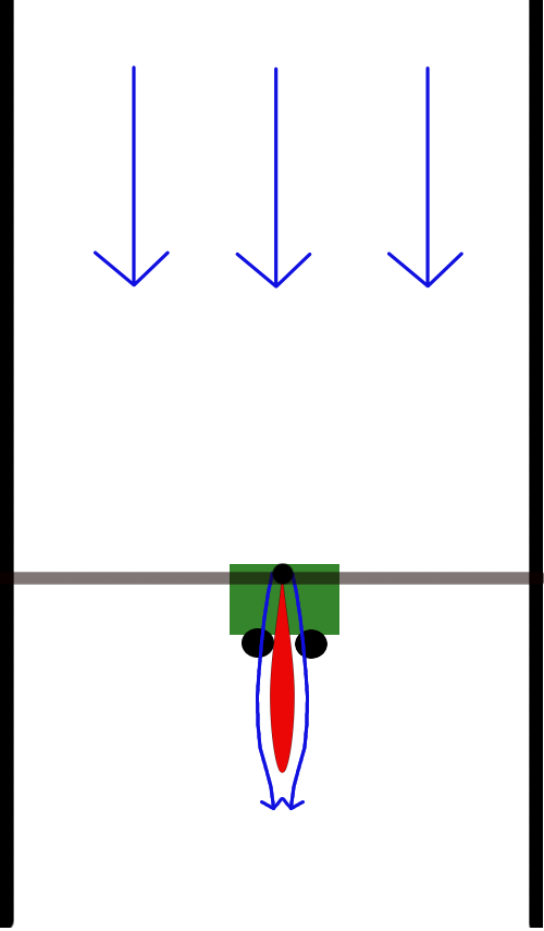
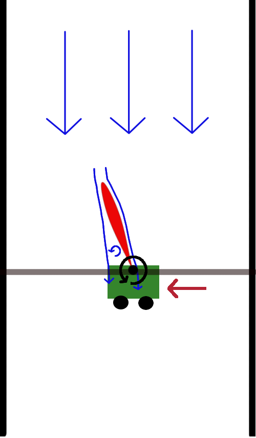
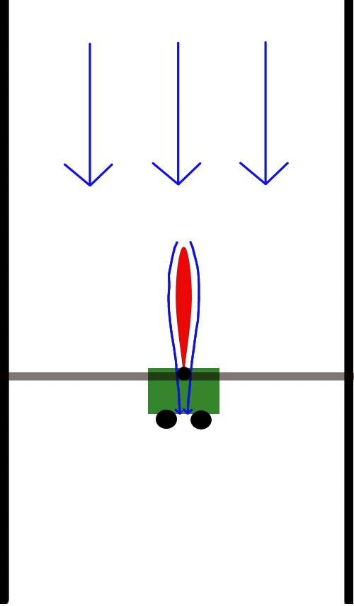
In a series of experiments, first we attempted to stabilize the system using an LQR controller derived with an approximate model (using flat-plate theory). This controller didn't perform well, but was just good enough to collect relevant data in the vicinity of the unstable fixed point. Then we fit a linear model, recomputed the LQR controller using the model, and got notably better performance.
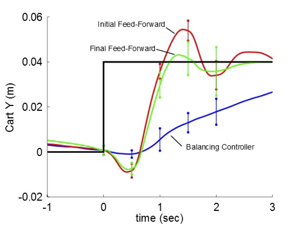
To investigate more aggressive maneuvers we considered making a rapid step change in the desired position of the cart (like a fighter jet rapidly changing altitude). Using only the time-invariant LQR balancing controller with a shifted set point, we naturally observed a very slow step-response. Using trajectory optimization on the time-invariant linear model used in balancing, we could do much better. But we achieved considerably better performance by iteratively fitting a time-varying linear model in the neighborhood of this trajectory and performing model-based ILC.
These experiments were quite beautiful and very visual. They went
on from here to consider the effect of stabilizing against incoming
vortex disturbances using real-time perception of the oncoming fluid.
If you're at all interested, I would encourage you to check out John
Robert's thesis
Compression using the dominant eigenmodes
For high-dimensional state or input vectors, one can use singular
value decomposition (SVD) to solve this least-squares problem using
only the dominant eigenvalues (and corresponding eigenvectors) of $\bA$
Linear dynamics in a nonlinear basis
A potentially useful generalization that we can consider here is identifying dynamics that evolve linearly in a coordinate system defined by some (potentially high-dimensional) basis vectors $\phi(\bx).$ In particular, we might consider dynamics of the form $\dot\bphi = \pd{\bphi}{\bx} \dot\bx = \bA \bphi(x).$ Much ado has been made of this particular form, due to the connection to Koopman operator theory that we will discuss briefly below. For our purposes, we also need a control input, so might consider a form like $\dot\bphi = \bA \bphi(x) + \bB \bu.$
Once again, thanks to the maturity of least-squares, with this approach it is possible to include list many possible basis functions, then use sparse least-squares and/or the modal decomposition to effectively find the important subset.
Note that multibody parameter estimation described above is not this, although it is closely related. The least-squares lumped-parameter estimation for the manipulator equations uncovered dynamics that were still nonlinear in the state variables.
From input-output data (the state-realization problem)
In the more general form, we would like to estimate a model of the
form \begin{gather*} \bx[n+1] = \bA \bx[n] + \bB \bu[n] + \bw[n]\\ \by[n]
= \bC \bx[n] + {\bf D} \bu[n] + \bv[n]. \end{gather*} Once again, we
will apply least-squares estimation, but combine this with the famous
"Ho-Kalman" algorithm (also known as the "Eigen System Realization" (ERA)
algorithm)
First, observe that \begin{align*} \by[0] =& \bC\bx[0] + {\bf D}\bu[0]
+ \bv[0], \\ \by[1] =& \bC(\bA\bx[0] + \bB\bu[0] + \bw[0]) + {\bf
D}\bu[1] + \bv[1], \\ \by[n] =& \bC\bA^n\bx[0] + {\bf D}\bu[n] + \bv[n] +
\sum_{k=0}^{n-1}\bC\bA^{n-k-1}(\bB\bu[k] + \bw[k]). \end{align*} For the
purposes of identification, let's write $\by[n]$ as a function of the most
recent $N+1$ inputs (for $k \ge N$): \begin{align*}\by[n] =&
\begin{bmatrix} \bC\bA^{N-1}\bB & \bC\bA^{N-2}\bB & \cdots & \bC\bB &
{\bf D}\end{bmatrix} \begin{bmatrix} \bu[n-N] \\ \bu[n-N+1] \\ \vdots \\
\bu[n] \end{bmatrix} + {\bf \delta}[n] \\ =& {\bf G}[n]\bar\bu[n] + {\bf
\delta}[n] \end{align*} where ${\bf \delta}[n]$ captures the remaining
terms from initial conditions, noise and control inputs before the
(sliding) window. ${\bf G}[n] = \begin{bmatrix} \bC\bA^{N-1}\bB &
\bC\bA^{N-2}\bB & \cdots & \bC\bB & {\bf D}\end{bmatrix},$ and
$\bar\bu[n]$ represents the concatenated $\bu[n]$'s from time $n-N$ up to
$n$. Importantly we have that ${\bf \delta}[n]$ is uncorrelated with
$\bar\bu[n]$: $\forall k > n$ we have $E\left[\bu_k {\bf \delta}_n
\right] = 0.$ This is sometimes known as Neyman orthogonality, and it
implies that we can estimate ${\bf G}$ using simple least-squares
$\hat{\bf G} = \argmin_{\bf G} \sum_{n \ge N} \| \by_n - {\bf G}\bar\bu_n
\|^2.$
How should we pick the window size $N$? By Neyman orthogonality, we know that our estimates will be unbiased for any choice of $N \ge 0$. But if we choose $N$ too small, then the term $\delta[n]$ will be large, leading to a potentially large variance in our estimate. For stable systems, the $\delta$ terms will get smaller as we increase $N$. In practice, we choose $N$ based on the characteristic settling time in the data (roughly until the impulse response becomes sufficiently small).
If you've studied linear systems, ${\bf G}$ will look familiar; it is
precisely this (multi-input, multi-output) matrix impulse response, also
known as the "Markov parameters". In fact, estimating $\hat{\bf
G}$ may even be sufficient for control design, as it is closely-related to
the parameterization used in disturbance-based feedback for
partially-observable systems
It is important to realize that many system matrices, $\bA, \bB, \bC,$
can describe the same input-output data. In particular, for any
invertible matrix (aka similarity
transform), ${\bf T}$, the system matrices $\bA, \bB, \bC$ and $\bA',
\bB', \bC'$ with, $$\bA' = {\bf T}^{-1} \bA {\bf T},\quad \bB' = {\bf
T}^{-1} \bB,\quad \bC' = \bC{\bf T},$$ describe the same input-output
behavior. The Ho-Kalman algorithm returns a balanced realization.
A balanced realization is one in which we have effectively applied a
similarity transform, ${\bf T},$ which makes the controllability and
observability Grammians equal and diagonal
Note that $\hat{\bf D}$ is the last block in $\hat{\bf G}$ so is
extracted trivially. The Ho-Kalman algorithm tells us how to extract
$\hat\bA, \hat\bB, \hat\bC$, with another application of the SVD on
suitably constructed data matrices (see e.g.
Ho-Kalman identification of the cart-pole from keypoints
Let's repeat the cart-pole example. But this time, instead of getting observations of the joint position and velocities directly, we will consider the problem of identifying the dynamics from a camera rendering the scene, but let us proceed thoughtfully.
The output of a standard camera is an RGB image, consisting of 3 x
width x height real values. We could certainly columnate these into a
vector and use this as the outputs/observations, $y(t)$. But I don't
recommend it. This "pixel-space" is not a nice space. For example,
you could easily find a pixel that has the color of the cart in one
frame, but after an incremental change in the position of the cart, now
(discontinuously) takes on the color of the background. Deep learning
has given us fantastic new tools for transforming raw RGB images into
better "feature spaces", that will be robust enough to deploy on real
systems but can make our modeling efforts much more tractable. My
group has made heavy use of "keypoint networks"
The existence of these tools makes it reasonable to assume that we have observations representing the 2D positions of some number of "key points" that are rigidly fixed to the cart and to the pole. The location of any keypoint $K$ on a pole, for instance, is given by the cart-pole kinematics: $${}^{W}{\bf p}^{K} = \begin{bmatrix} x \\ 0 \end{bmatrix} + \begin{bmatrix} \cos\theta & -\sin\theta \\ \sin\theta & \cos\theta \end{bmatrix} {}^{P}{\bf p}^{K},$$ where $x$ is the position of the cart, and $\theta$ is the angle of the pole. I've used Monogram notation to denote that ${}^{P}{\bf p}^{K}$ is the Cartesian position of a point $A$ in the pole's frame, $P$, and ${}^{W}{\bf p}^{K}$ is that same position in the camera/world frame, $W$. While it is probably unreasonable to linearize the RGB outputs as a function of the cart-pole positions, $x$ and $\theta$, it is reasonable to approximate the keypoint positions by linearizing this equation for small angles.
You'll see in the example that we recover the impulse response quite nicely.

The big question is: does Ho-Kalman discover the 4-dimensional state vector that we know and like for the cart-pole? Does it find something different? We would typically choose the order by looking at the magnitude of the singular values of the Hankel data matrix. In this example, in the case of no noise, you see clearly that 2 states describe most of the behavior, and we have diminishing returns after 4 or 5:

As an exercise, try adding process and/or measurement noise to the system that generated the data, and see how they effect this result.
Adding stability constraints
Details coming soon. See, for instance
Autoregressive models
Another important class of linear models predict the output directly from a history of recent inputs and outputs: \begin{align*} \by[n+1] =&\bA_0 \by[n] + \bA_1 \by[n-1] + ... + \bA_k \by[n-k] \\ & + \bB_0\bu[n] + \bB_1 \bu[n-1] + ... \bB_k \bu[n-k]\end{align*} These are the so-called "AutoRegressive models with eXogenous input (ARX)" models. The coefficients of ARX models can be fit directly from input-output data using linear least squares.
While it is certainly possible to think of these models as state-space models, where we collect the finite history $\by$ and $\bu$ (except not $\bu[n]$) into our state vector. But this is not necessarily a very efficient representation; the Ho-Kalman algorithm might be able to find a much smaller state representation. This is particularly important for partially-observable systems that might require a very long history, $k$.
A state-space model that would be inefficient in ARX
An ARX model of cart-pole keypoint dynamics
Statistical analysis of learning linear models
Identification of finite (PO)MDPs
There is one more case that we can understand well: when states, actions, and observations (and time) are all discrete. Recall that in the very beginnings of our discussion about optimal control and dynamic programming, we used graph search and discretization of the state space to give a particularly nice version of the value iteration algorithm. In general, we can write the stochastic dynamics using conditional probabilities: $$\Pr(s[n+1] | s[n], a[n]), \qquad \Pr(o[n] | s[n], a[n]),$$ where I've (again) used $s$ for discrete states, $a$ for discrete actions, and $o$ for discrete observations. With everything discrete, these conditional probabilities are represented naturally with matrices/tensors. We'll use the tensors $T_{ijk} \equiv \Pr(s[n+1] = s_i | s[n] = s_j, a[n] = a_k)$ to denote the transition matrix, and $O_{ijk} \equiv \Pr(o[n] = o_i | s[n] = s_j, a[n] = a_k)$ for the observation matrix.
From state observations
Following analogously to our discussion on linear dynamical systems, the first case to understand is when we have direct access to state and action trajectories: $s[\cdot], a[\cdot]$. This corresponds to identifying a Markov chain or Markov decision process (MDP). The transition matrices can be extracted directly from the statistics of the transitions: $$T_{ijk} = \frac{\text{number of transitions to } s_i\text{ from }s_j, a_k}{\text{total number of transitions from }s_j, a_k}.$$ Not surprisingly, for this estimate to converge to the true transition probabilities asymptotically, we need the identification (exploration) dynamics to be ergodic (for every state/action pair to be visited infinitely often).
For large MDPs, analogous to the modal decomposition that we described for linear dynamical systems, we can also consider factored representations of the transition matrix. [Coming soon...]
Identifying Hidden Markov Models (HMMs)
Neural network models
If multibody parameter estimation, linear system identification, and finite state systems are the first pillars of system identification, then (at least these days) deep learning is perhaps the last major pillar. It's no coincidence that I've put this section just after the section on linear dynamical systems. Neural networks are powerful tools, but they can be a bit harder to think about carefully. Thankfully, we'll see that many of the basic lessons and insights from linear dynamical systems still apply here. In particular, we can follow the same progression: learning the dynamics function directly from state observations, learning state-space models from input-output data (with recurrent networks), and learning input-output (autoregressive) models with feedforward networks using a history of outputs.
Deep learning tools allow us to quite reliably tune the neural networks to fit our training data. The major challenges are with respect to data efficiency/generalization, and with respect to actually designing planners / controllers based on these models that have such complex descriptions.
Generating training data
One extremely interesting question that arises when fitting rich nonlinear models like neural networks is the question of how to generate the training data. You might have the general sense that we would like data that provides some amount of "coverage" of the state space; this is particularly challenging for underactuated systems since we have dynamic constraints restricting our trajectories in state space.
For multibody parameter estimation we discussed using the condition number of the data matrix as an explicit objective for experiment design. This was a luxury of using linear least-squares optimization for the regression and it takes advantage of the specialized knowledge we have from the manipulator equations about the model structure. Unfortunately, we don't have an analogous concept in the more general case of nonlinear least squares with general function approximators. This approach also works for identifying linear dynamical systems. The challenge is here perhaps considered less severe since for linear models in the noise-free case even data generated from the impulse response is sufficient for identification.
This topic has received considerable attention lately in the context
of model-based reinforcement learning (e.g.
From state observations
State-space models from input-output data (recurrent networks)
Input-output (autoregressive) models
You might have heard about a neural network model called the
Transformer
Particle-based models
Object-centric models
Modeling stochasticity
Control design for neural network models
Alternatives for nonlinear system identification
Identification of hybrid systems
Task-relevant models
As discussed briefly in the introduction, the standard objective for system identification is to match the input-output behavior of a dynamical system. Certainly if we can find a model that predicts all outputs perfectly, then this model should be sufficient for making optimal decisions. But when we cannot make perfect predictions, due to limited data and/or limited model representation power, then the relative cost placed on predicting different outputs becomes important. This feels particularly important when the observations come from a camera -- in most cases predicting every pixel in the scene accurately is not the right objective for a robot trying to use the camera to accomplish a particular task.
Fortunately, the problem of learning task-relevant models or "learning state representations" has become a darling of the machine learning community. There are a lot of smart people thinking about the problem and the field has made considerable progress in the last years. In the immense volume of papers, I think there are a few really core ideas.
What makes a good state representation for control? Two defining properties are: 1) it should be observable, and 2) it should be sufficient for making optimal decisions. In other words, if $\bz[n]$ is the state of the dynamic controller (which we can think of as an observer of the learned state representation), then we would like that the optimal policy given this state to take the same action as an optimal policy which uses the entire available history: $$\pi^*(\bz[n]) \approx \bar\pi^*(\by[n], \by[n-1], \by[n-2], ..., \bu[n-1], \bu[n-2], ...).$$ Certainly the belief state, which is by definition a sufficient statistic for predicting future observations, has this property. But much more minimal representations may also be sufficient. So a third, slightly more tenuous property of a good state representation is that we would like it to be tractable for learning, representation, and decision making.
Being sufficient for making optimal control decisions is a difficult
objective because it couples the problem of representation learning / system
identification with the problem of control design. How can we know what the
optimal action is without solving the optimal control problem? This is one
reason that imitation learning
A closely related idea would ask for the representation to be sufficient to predict the optimal value function (rather than the optimal action). Certainly if we have a model and a value function that is consistent with that model, then this would be sufficient for making optimal decisions. But it should be noted that there are cases where predicting the optimal cost-to-go is actually harder than predicting the optimal action. Imagine an agent in a grid world that can traverse one of two corridors and has learned that the left corridor always has more reward than the right. Predicting the precise amount of reward that will be obtained when moving down the left corridor is not needed to choose the optimal action. Predicting optimal values also does not break the "chicken-and-the-egg" problem (how can you know the optimal values until you have an optimal policy?), but may have more subtle merits in terms of representation or learning efficiency.
One proposal which does fundamentally break the chicken-and-the-egg
problem is given by
Approximate information states are themselves closely related to prior
work on "state aggregation" in MDPs via the so-called "bisimulation metrics".
The basic idea is that if the future outcomes from two states are
indistinguishable, then these states can be aggregated into a single state,
thus reducing the state space. See
Interestingly, the famous work by DeepMind on MuZero
This area is moving fast; I will try to update this section as results appear, and will give some worked out examples soon.
Exercises
Linear System Identification with different objective functions
Consider a discrete-time linear system of the form $$x[n+1] = Ax[n]+Bu[n]$$ where $x[n]\in\mathbf{R}^p$ and $u[n]\in\mathbf{R}^q$ are state and control at step $n$. The system matrix $A\in\mathbf{R}^{p\times p}$ and $B\in\mathbf{R}^{p\times q}$ are unknown parameters of the model, and your task is to identify the parameters given a simulated trajectory. Using the trajectory simulation provided in , implement the solution for the following problems.
- Identify the model parameters by solving $$\min_{A, B}\sum_{n=0}^{N-1}\lVert x[n+1] - Ax[n] -Bu[n] \rVert_2^2.$$
- Identify the model parameters by solving $$\min_{A, B}\sum_{n=0}^{N-1}\lVert x[n+1] - Ax[n] -Bu[n] \rVert_{\infty}.$$
- Identify the model parameters by solving $$\min_{A, B}\sum_{n=0}^{N-1}\lVert x[n+1] - Ax[n] -Bu[n] \rVert_1.$$
System Identification for the Perching Glider
In this exercise we will use physically-inspired basis functions to fit the nonlinear dynamics of a perching glider. , you will need to implement least-squares fitting and find the best set of basis functions that describe the dynamics of the glider. Take the time to go through the notebook and understand the code in it, and then answer the following questions. The written question will also be listed in the notebook for your convenience.
- Work through the coding sections in the notebook.
- All of the basis configurations we tested used at most 3 basis functions to compute a single acceleration. If we increase the number of basis functions used to compute a single acceleration to 4, the least-squares residual goes down. Why would we limit ourselves to 3 basis functions if by using more we can generate a better fit?